Production, Costs, and Economies of Scale
Matthew Williams
||10 min readCost CurvesCSEC EconomicsEconomies of ScaleLong RunPaper 01Paper 02Production FunctionSection 2Short Run
Short-run and long-run production, total and marginal product, fixed and variable costs, average and marginal cost, cost curves, economies and diseconomies of scale.
A firm's decisions about how much to produce depend on two things: how much output it can squeeze from its inputs (its production function) and how much that production costs. These two sides are closely linked — the shape of cost curves follows directly from the behaviour of output.
Short Run vs Long Run
In economics, the short run and long run are not fixed calendar periods. They are defined by whether inputs can be varied.
Short run: at least one factor of production is fixed — it cannot be changed regardless of how much the firm wants to produce. For most firms, capital (factories, machinery) is the fixed factor in the short run. Labour and raw materials are variable.
Long run: all factors of production are variable. The firm can change the size of its factory, buy new machines, or change the scale of its entire operation. There are no fixed factors.
The Production Function
The production function describes the relationship between inputs and outputs. It shows the maximum output attainable from a given combination of inputs, at a given state of technology.
In the short run, the firm adds units of a variable input (labour) to a fixed input (capital). The result is captured by three measures:
| Measure | Definition | Formula |
|---|---|---|
| Total Product (TP) | Total output produced by all units of the variable input | — |
| Average Product (AP) | Output per unit of variable input | AP = TP ÷ L |
| Marginal Product (MP) | Change in total output from adding one more unit of variable input | MP = ΔTP ÷ ΔL |
The Law of Diminishing Returns
As successive units of a variable input are added to a fixed input, the marginal product will eventually begin to fall. This is the law of diminishing marginal returns (or diminishing returns).
It applies only in the short run, because in the long run all inputs can be varied.
Example
A firm has 5 machines (fixed). It hires workers one at a time:
| Workers | TP | MP | AP |
|---|---|---|---|
| 0 | 0 | — | — |
| 1 | 14 | 14 | 14.0 |
| 2 | 26 | 12 | 13.0 |
| 3 | 36 | 10 | 12.0 |
| 4 | 44 | 8 | 11.0 |
| 5 | 50 | 6 | 10.0 |
| 6 | 54 | 4 | 9.0 |
| 7 | 56 | 2 | 8.0 |
| 8 | 56 | 0 | 7.0 |
| 9 | 54 | -2 | 6.0 |
Marginal product falls from the second worker onwards because each additional worker has less capital to work with. Beyond 8 workers, MP is negative and TP falls — the workers get in each other's way.
Three Stages of Production
- Stage 1 — MP is above AP; both MP and AP are rising. Fixed factor is underutilised.
- Stage 2 — MP falls below AP; AP is declining; MP is still positive; TP is still rising. This is the rational stage for production.
- Stage 3 — MP is negative; TP is falling. The firm is using too many variable inputs.
A profit-maximising firm produces in Stage 2, where TP is rising but at a decreasing rate, up to the point where MP = 0.
Cost Functions
Fixed and Variable Costs
| Cost | Definition | Behaviour |
|---|---|---|
| Total Fixed Cost (TFC) | Costs that do not change with output | Constant at every level of output, including zero |
| Total Variable Cost (TVC) | Costs that vary directly with output | Zero when output is zero; rises as output rises |
| Total Cost (TC) | TFC + TVC | Always above TFC; TC = TFC when Q = 0 |
Examples of fixed costs: rent on factory, insurance premiums, loan repayments, management salaries. Examples of variable costs: raw materials, hourly labour, electricity for machines, packaging.
Unit Costs
| Cost | Definition | Formula |
|---|---|---|
| Average Fixed Cost (AFC) | Fixed cost per unit | AFC = TFC ÷ Q |
| Average Variable Cost (AVC) | Variable cost per unit | AVC = TVC ÷ Q |
| Average Total Cost (ATC) | Total cost per unit | ATC = TC ÷ Q = AFC + AVC |
| Marginal Cost (MC) | Cost of producing one additional unit | MC = ΔTC ÷ ΔQ |
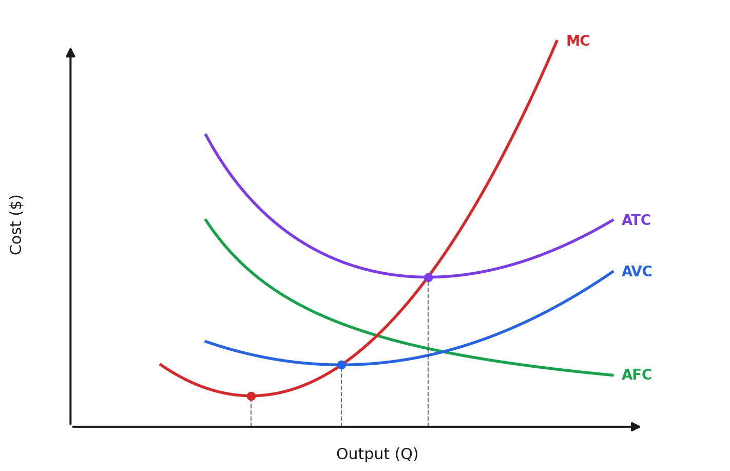
AFC always falls as output rises — the fixed cost is spread over more and more units.
AVC, ATC, and MC are all U-shaped in the short run. They fall initially as rising marginal product means each additional unit costs less, then rise as diminishing returns set in.
The relationship between MC and average costs:
- When MC is below ATC, it pulls ATC downward.
- When MC is above ATC, it pulls ATC upward.
- MC crosses ATC and AVC at their minimum points.
Exam Tip
A common exam question gives a table of TC values and asks you to calculate MC or ATC. MC = change in TC when output rises by 1; ATC = TC ÷ Q. Marginal cost crosses average total cost at its lowest point — use this to check your numbers.
Example
From a production schedule:
| Q | TC | ATC | MC |
|---|---|---|---|
| 0 | 100 | — | — |
| 1 | 190 | 190 | 90 |
| 2 | 270 | 135 | 80 |
| 3 | 330 | 110 | 60 |
| 4 | 380 | 95 | 50 |
| 5 | 450 | 90 | 70 |
| 6 | 540 | 90 | 90 |
| 7 | 630 | 90 | 90 |
| 8 | 800 | 100 | 170 |
ATC reaches its minimum of 90 (Q ≈ 6), consistent with the rule that MC = ATC at the ATC minimum.
Long-Run Production: Returns to Scale
In the long run, all inputs are variable. When a firm increases all its inputs by the same proportion, its output may respond in three ways:
| Returns to Scale | What happens | Effect on LRAC |
|---|---|---|
| Increasing returns to scale | Output rises by a larger proportion than inputs | LRAC falls (economies of scale) |
| Constant returns to scale | Output rises by the same proportion as inputs | LRAC is constant |
| Decreasing returns to scale | Output rises by a smaller proportion than inputs | LRAC rises (diseconomies of scale) |
Economies of Scale
Economies of scale occur when a firm's long-run average cost (LRAC) falls as it expands its scale of production.
Internal Economies of Scale
These arise from the growth of the individual firm:
| Type | Explanation |
|---|---|
| Technical | Larger machines are often more efficient per unit; indivisibilities mean a large firm can use specialised equipment fully |
| Marketing | Buying in bulk reduces input costs; advertising costs spread over larger output |
| Financial | Larger firms can borrow at lower interest rates because they are seen as lower-risk |
| Managerial | Can hire specialist managers rather than one person doing everything |
| Risk-bearing | Diversifying across products and markets reduces the impact of any one failure |
External Economies of Scale
These arise from the growth of the entire industry, benefiting individual firms within it. For example, when the aluminium industry expands in a region, specialist suppliers set up nearby, reducing costs for all producers.
Diseconomies of Scale
Diseconomies of scale occur when LRAC rises as the firm grows beyond an optimal size. The main causes are management problems:
- Communication breakdown — information becomes distorted as it passes through more layers of management.
- Coordination problems — aligning the actions of many specialised departments becomes difficult.
- Worker alienation — in very large organisations, workers feel anonymous and less motivated.
- Slower decision-making — consensus in large management teams takes longer to reach.
- Over-specialisation boredom — highly repetitive roles reduce motivation and job satisfaction.
The minimum efficient scale (MES) is the lowest output level at which the firm has fully exploited all economies of scale — where LRAC first reaches its minimum.
Remember
Economies of scale reduce average cost as output rises. Diseconomies of scale increase average cost as the firm grows too large. The primary cause of diseconomies is management and coordination failure, not diminishing returns (which is a short-run phenomenon).